

This time, we’ll discuss tracking analysis, one of the most commonly used applications of FFT analyzers for measuring sound and vibration. Tracking analysis continuously examines how amplitude levels change in response to the rotational speed of a rotating body. Its primary purpose is to determine the relationship between a rotating machine’s resonant frequencies and its rotational speed. Here, we’ll briefly explain the measurement principles behind tracking analysis, its relationship to FFT, and some points to keep in mind.
The frequency spectra of sounds and vibrations generated by rotating machinery, such as engines, motors, and power plants, contain not only the fundamental rotational-speed component but also forced-vibration components at integer multiples of the rotational speed, as well as components caused by resonance in the machinery’s constituent parts, because the excitation forces depend on rotational speed. In addition, the rotational speed of such machinery is not necessarily constant. For equipment with a wide operating-speed range, such as an automobile, the signal components that appear as the rotational speed changes also vary across a broad frequency range. Tracking analysis determines, for example, the rotational speed at which a component of the machinery resonates, or which multiple of the rotational speed is resonating.
detector
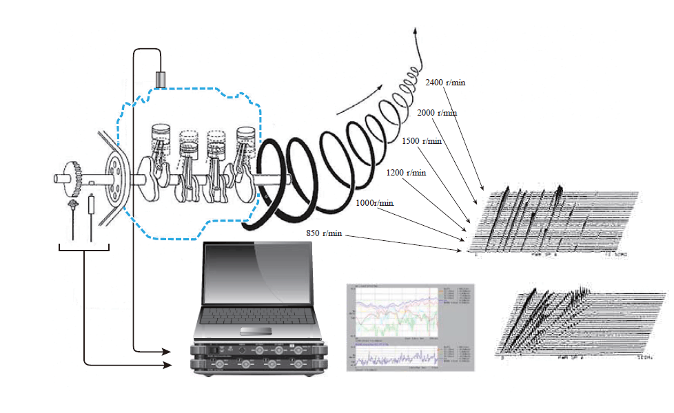
[{"source":"Figure 1: Illustration of tracking analysis"}]
Figure 1 shows a conceptual diagram of tracking analysis. As illustrated, tracking analysis adds rotational speed as a parameter to the conventional frequency spectrum (a two-dimensional plot of frequency and amplitude), resulting in a three-dimensional plot.
The excitation force components of a rotating body generally occur at the rotational speed and its integer multiples, and their frequencies change in tandem when the rotational speed changes. The frequency corresponding to the rotational speed is called the first-order rotational component. For example, at 1,200 r/min, dividing the rotational speed by 60 gives a first-order frequency of 20 Hz; at 1,800 r/min, it is 30 Hz. Similarly, the nth-order component has a frequency n times as high.
Table 1. Rotational Speed and Rotational Order Frequencies (Examples)
| Rotational speed (r/min) | 1st-order component (Hz) | Second-order component (Hz) | nth component (Hz) |
| 600 | 10 | 20 | 10n |
| 1200 | 20 | 40 | 20n |
| 1800 | 30 | 60 | 30n |
| 2400 | 40 | 80 | 40n |
| 3000 | 50 | 100 | 50n |
トラッキング解析を行うためには、回転体の回転情報が必要となり、図 1 にあるように回転体に回転センサーを取り付け、FFT アナライザヘ通常パルス信号や交流信号を入力します。例えば、図1 の左側センサーは、検出歯車に近接させ磁気抵抗の変化からの誘起電圧を出力する電磁式回転検出器(交流信号が出力される)やホール素子を使った磁電式回転検出器(パルス信号が出力される)です。右側は、回転シャフトに反射テープを貼り付けて1パルス/1回転を検出する非接触式ハンディタコメータの例です。(注意:図1には、例として2つの回転センサーが描いてありますが、実際はどちらか1つを使うことになります。)
An example of the rotation settings in the FFT analyzer is shown in Figure 2.
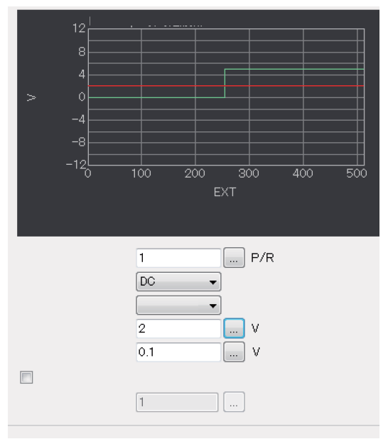
[{"source":"Figure 2 Example of setting the conditions for rotational input on an FFT analyzer"}]
①パルス数
1 回転あたりのパルス数を入力
検出歯車の数 60 であれば、60 を入力
1 つの反射テープであれば、1 を入力
②カップリング
交流信号ならば、AC
パルス信号ならば、DC
③エッジ
立ち上がり/立ち下がり 通常どちらでも OK
④検出レベル
波形生成用電圧レベル(グラフの赤ライン)
DC カップリングでパルス波形ならば、2 V 程度に
⑤ヒステリシス
誤動作防止用のレベル、通常は 0.1 V 程度
⑥ハードウェア分周と分周数
通常はオフでいいですが、センサーによって FFT アナライザに入力される回転情報の周波数が 3 kHz を超えるようでしたらオンして適切な分周数を入力して下さい
外部からの回転情報に連動してその回転速度での次数成分をトラックしていくことがトラッキング解析の主たる機能ですが、現在 FFT アナライザで次数成分をトラックする方法として、次数比分析と通常の周波数分析との2つ使われています。
次数比分析は、外部からの回転情報からサンプリングパルスを作成して入力してくる音や振動の時間信号を回転速度に連動したサンプリング周波数でサンプルすることにより、回転速度に関係なく一定の幅の次数成分の周波数分析を行う手法です。このことにより、次数成分が回転速度に関わらず固定のスペクトルの分析ラインとなりトラックしやすくなります。また、FFT の時間窓の誤差も少なくすることができます。この次数比分析を使う手法を定比トラッキングと呼びます。
それに対して、通常の周波数分析を使う方法は、分析自体は固定のサンプリング周波数を使い(すなわち通常の周波数レンジを設定する)、その時の回転速度に連動して毎回回転次数成分の周波数が変化するので対応する分析ラインをサーチする必要があります。また、その次数成分の周波数は非同期なので、分析幅にピッタリ合わず時間窓の影響を大きく受けます。この通常の周波数分析を使う手法を定幅トラッキングと呼びます。
図3は、3次元表示に対応したカラーマップで表現した、上記の2つの手法を比較したものです。
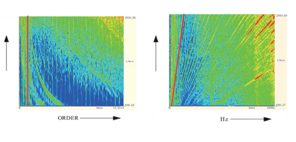
Figure 3 Example comparing constant-ratio tracking and constant-bandwidth tracking
Constant-ratio horizontal axis: constant order (12.5 order in this example)
Constant-bandwidth horizontal axis: constant frequency (500 Hz in this example)
Amplitude magnitude is represented by color
As shown in Figure 3, at a constant rotational speed, a specific order component appears as a line parallel to the rotational-speed axis (the red line in the figure) and corresponds to a fixed analysis line in the FFT. At a constant bandwidth, a specific order component appears as a sloping line proportional to rotational speed (the red line in the figure), showing that its frequency changes continuously as the rotational speed varies.
そして、この次数成分に着目して、横軸を回転速度表示したものを回転トラッキング線図と呼びます。図4は、4つの次数を重ね書き表示した例です。
-
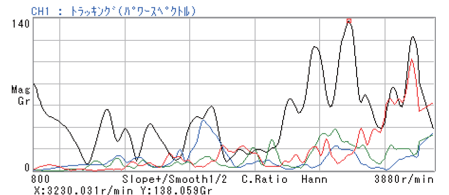
Figure 4 Example of a rotational tracking diagram (overlay of four orders)
Horizontal axis: Rotational speed Vertical axis: Sound or vibration amplitude
This section explains the difference in analysis bandwidth (frequency resolution) between constant-ratio tracking and constant-bandwidth tracking. With constant-ratio tracking, the signal is sampled so that the FFT time window (for example, 1,024 samples) always captures an integer number of cycles of the rotational fundamental frequency, regardless of rotational speed. As a result, frequency resolution is proportional to the rotational fundamental frequency. Because the frequency resolution maintains a constant ratio, this method is called constant-ratio tracking. By contrast, constant-bandwidth tracking uses a conventional frequency range, so frequency resolution remains constant regardless of rotational speed.
次に、定比トラッキングの使用上の注意点を述べます。
定比トラッキング時の次数比分析では、通常回転速度に対応した外部からのパルスを分周逓倍してサンプリング周波数を作っていますが(最近のFFT では、ディジタルフィルタとリサンプリング手法で行なっています)、最大分析次数と 1 回転 1 パルス数を基準としたパルス逓倍率は、通常の周波数分析における周波数レンジとサンプリング周波数と同じく、2.56 のファクタとなります。
すなわち

となります。(表2)
表2 最大分析次数と逓倍率との関係
| maximum number of analyses | 6.25 | 12.5 | 25 | 50 | 100 | 200 | 400 | 800 | 1600 |
| Transmission ratio (at 1 P/R) | 16 | 32 | 64 | 128 | 256 | 512 | 1024 | 2048 | 4096 |
As the maximum analysis order increases, the processing load required to generate the sampling frequency in real time becomes heavier, limiting the upper rotational speed that can be analyzed, as shown in Table 3.
Table 3. Upper Limit of Analyzable Rotational Speed by Maximum Number of Analyses
| maximum number of analyses | Measurement rotational speed range | Sampling |
| 6.25 | 300~240000 r/min | 16 points per rotation |
| 12.5 | 200~192000 r/min | 32 points per revolution |
| 25 | 150~96000 r/min | 64 points per revolution |
| 50 | 150~48000 r/min | 128 points per revolution |
| 100 | 150~24000 r/min | 256 points per revolution |
| 200 | 100~12000 r/min | 512 points/1 rotation |
| 400 | 100~6000 r/min | 1024 points/1 rotation |
| 800 | 100~3000 r/min | 2048 points per rotation |
| 1600 | 100~1500 r/min | 4096 points/revolution |
A point to note when using fixed-width tracking is that the maximum analysis rotational speed and maximum analysis order are limited by the frequency range being analyzed (which is fixed).
Let Nmax be the maximum rotational speed that can be analyzed, Omax the maximum analysis order, and Fr the frequency range.

For example, in the 1 kHz range, at 3,000 r/min, analysis is possible only up to the 20th order.
A general point to keep in mind when performing tracking analysis with an FFT analyzer is the speed (rate) at which the rotational speed changes. FFT analysis calculates the average amplitude over the time window, whereas the sound and vibration signals of rotating machinery are considered non-stationary over long time spans. If the rotational speed changes rapidly within the time window, accurate amplitude information cannot be obtained. This is especially important at low rotational speeds in constant-ratio tracking, because the time window in constant-ratio tracking increases in inverse proportion to the rotational speed. Another point to keep in mind regarding changes in rotational speed is that tracking analysis determines the current rotational speed in real time from the input pulse signal. If the rotational speed changes too quickly, data may not be acquired at the configured rotational speed intervals.
Table 4 summarizes the characteristics of constant-ratio tracking and constant-bandwidth tracking discussed so far.
Finally, here is an example of three-dimensional data visualization of vibration data from a car engine analyzed using constant-ratio and constant-bandwidth tracking.
Figure 4 shows a measurement example using order tracking, making it easier to identify the characteristics of the order components. Figure 5 shows constant-bandwidth tracking; the second-order component produces results that are nearly identical to those from order tracking. Also, vibration increases where a certain frequency range coincides with a rotational order component, suggesting a resonance frequency.
["Table 4: Key Comparison of Fixed-Ratio Tracking and Fixed-Width Tracking"]
| Comparison item | Fixed-ratio type | Fixed-width type |
| Sampling | 外部 回転速度に同期してサンプリング周波数が変化する。 |
内部 回転速度に無関係に一定のサンプリング周波数でサンプルする。 |
| Analysis range | 最大分析次数 6.25、12.5、25、50、100、200、400、800 分析したい最大次数から選択する。 |
周波数レンジ 分析したい次数と回転速度から周波数レンジを選択する。最大次数が制限される。 |
| Order resolution (Δorder) | Constant at maximum analysis order/frequency resolution (Example) 0.125 at 50 orders and 400 lines |
As rotational speed increases, the maximum analysis order decreases, resulting in finer order resolution. |
| Frequency bandwidth (frequency resolution) | 回転速度に比例して大きくなる。(定比幅) | Constant regardless of rotational speed Frequency range / frequency resolution |
| How to track | Because it is only necessary to track a fixed number of lines analyzed by FFT, it responds well to rotational transformations It is easy to catch peaks corresponding to the order. (Unaffected by the time window) |
Calculate the frequency corresponding to a specific order for each instantaneous rotational speed, and track the band data around it. Since the order component does not align with the frequency resolution, synthesize it from the adjacent bands. (Significant influence from the time window) |
| Number of samples per revolution | Constant regardless of rotational speed. Maximum analysis order × 2.56 (= multiplication factor) |
It decreases in inverse proportion to the rotational speed. |
| Overall frequency band | 回転速度に比例してバンド幅は大きくなる。 | 周波数レンジそのもの、 回転速度に無関係で一定。 |
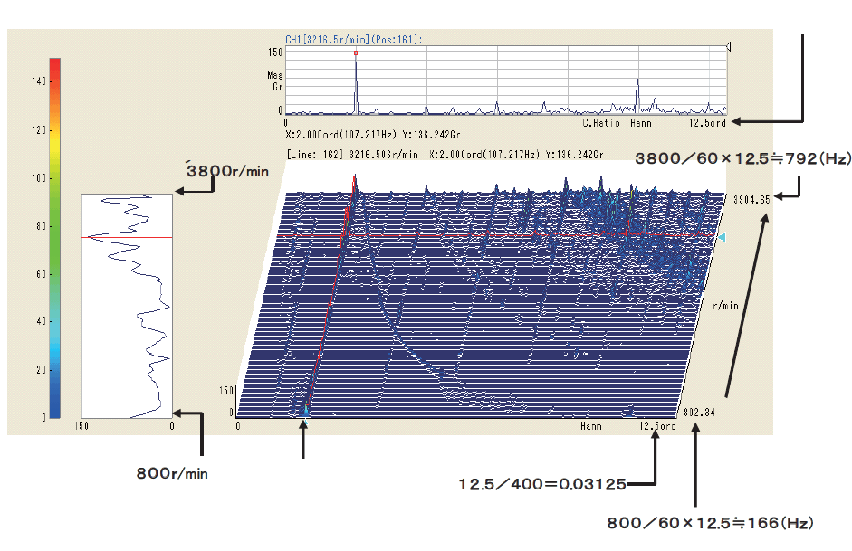
Figure 5. Example of Constant-Ratio Tracking Measurement
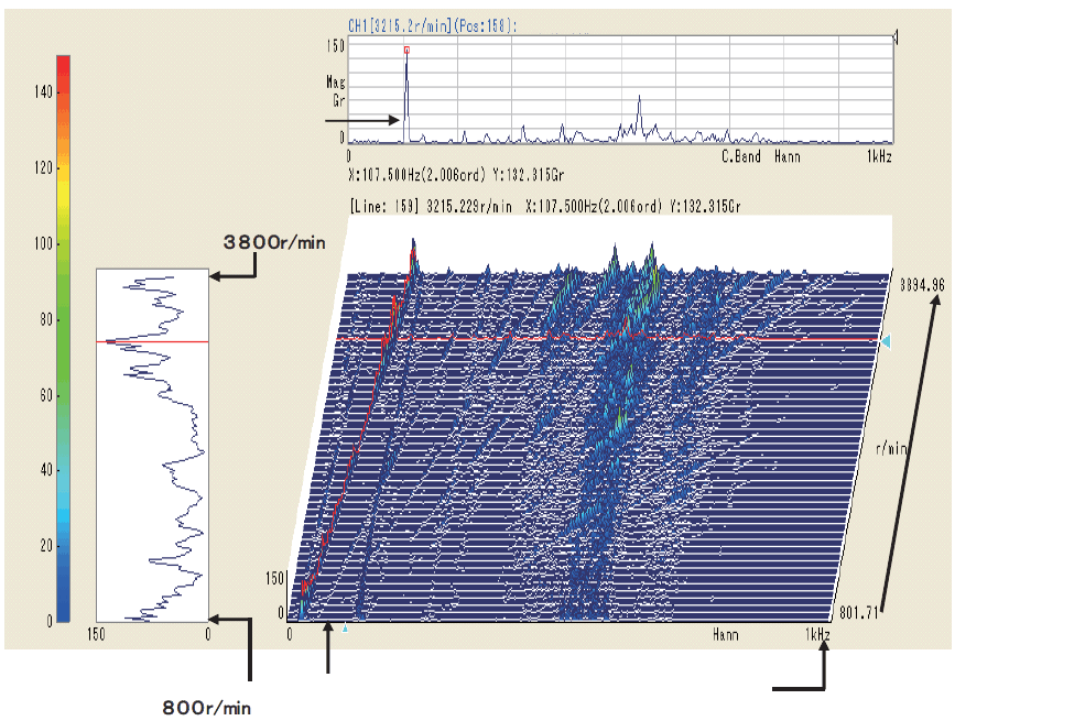
Resolution does not match
Figure 6: Example of Fixed-Width Tracking Measurement
[Keyword]
Tracking analysis, order, Electromagnetic Detector, Magneto-Electric Rotation Detector, handheld tachometer, order ratio analysis, frequency analysis, constant-ratio tracking, constant-bandwidth tracking, rotational tracking diagram, frequency division and multiplication, maximum analysis order
Reference
Ono Sokki Technical Report “Order Ratio Analysis and Tracking Analysis”
Ono Sokki Website Overview of Measuring Instruments for Rotating Machinery
Ono Sokki Website Overview of Handheld Tachometers (Revolution Counters)
(Excerpt from the email newsletter issued on November 21, 2017)


