Frequency Analysis from Basics (11) - Fourier Spectrum

So far, we have covered the fundamentals of Fourier series, Fourier transforms, and discrete Fourier transforms. From here on, we will discuss spectral analysis, one of their most important applications.

Breaking down complex signal waveforms, such as sound or vibration, into their basic frequencies (sine waves) and determining their strengths is called spectral analysis (or Fourier analysis). The most common way to perform this is by using Fourier transform techniques. Below, using basic waveforms, we explain how to calculate the discrete Fourier transform (DFT) and what the values on the vertical axis of the results represent.

First, let us restate the definitions of the Fourier series, Fourier transform, and discrete Fourier transform that we have discussed so far.

● Fourier Series

● Fourier Transform

● Discrete Fourier Transform (DFT)

In actual numerical computations, we work with finite-length digital data, so we use the DFT in Equation (3).

Here, we explain how to intuitively derive the finite-length DFT formula (3) from equation (2).
When the time waveform x(t) is sampled at N points with a sampling period τ (sampling frequency f, f = 1/τ), the finite time length T is T = Nτ. Also, the fundamental frequency is 1/T, and the discrete frequencies are k/T. Using these, we obtain the finite discretization of equation (2):

Here, omitting 1/T and τ and replacing the product with a sum gives:

Thus, the finite-length Fourier transform can be obtained using Equation (3).

X(f) (or X(k)) represents the magnitude (strength) of the frequency components contained in the time waveform x(t), and is called the Fourier spectrum. Since the Fourier spectrum is clearly a complex number;

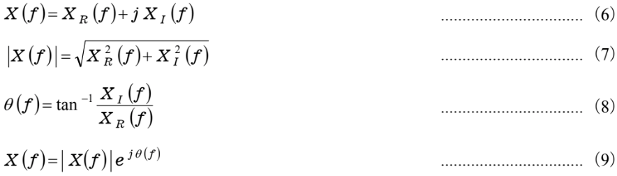
Here, |x(f)| is sometimes called the amplitude spectrum, and θ(f) the phase spectrum.
Thus, the Fourier spectrum is a complex number that contains amplitude and phase information for each frequency.

Next, we consider the dimensions of the magnitude of the Fourier spectrum.

When the Fourier transform of a finite-duration waveform x(t) is calculated using Equation (5), it is clearly an integration with respect to time. Therefore, the dimensions of X(f) are the product of the dimensions of the time-domain waveform and time. For example, if x(t) is measured in volts (V), the Fourier spectrum X(f) has units of V·s, and its value is proportional to the finite duration T.

For deterministic signals such as periodic signals, it is inconvenient for the values to change depending on the time window used for the calculation. Therefore, conventional FFT analyzers define the Fourier spectrum as the value divided by T. As explained in the Discrete Fourier Transform (DFT) column (Measurement Column, Newsletter No. 138), the DFT operation in Equation (5) treats the N-point data as a periodic time waveform whose fundamental period is N points. Thus, the “Fourier spectrum divided by T” is equivalent to the complex Fourier coefficients in Equation (1). In other words, as shown in Equation (10) of the Fourier Transform column (Measurement Column, Newsletter No. 130), the relationship between the complex Fourier coefficients and the Fourier spectrum obtained from the DFT is as follows (with the discrete arguments written explicitly):

will become.

Let’s try performing some actual numerical calculations using an FFT program included with commercially available spreadsheet software.

Consider a cosine waveform x(nτ) with k periods in a time window of length T (= Nτ);

Hereafter, as in Equation (11), the sampling period τ is omitted.

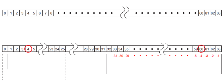
In Equation (11), for example, substituting N = 64 and k = 4 makes the time-domain signal x(n) a set of 64 discrete data points. Applying the FFT to these data yields a corresponding set of 64 frequency-domain data points (Figure 1, reproduced from the previous installment).

Time data (n =0,1,2,3, ….... ,63)

Frequency data (k =0,1,2,3, ….... ,63)

Positive frequency

Negative frequency

Frequency range on the
FFT analyzer

図1 DFT( FFT) における周波数領域のデータ並び(N = 64 の例)

In this example, the values from Table 1 are stored only at two positions in the frequency data sequence in Figure 1: k = 4 (positive frequency) and k = 60 (negative frequency), the two points circled in red. All other entries in the sequence are 0.

表1 式(11)に N = 64、k = 4 を代入した計算結果

frequency point (k)	real part	imaginary part
4 (positive frequency)		0
60 (negative frequency)		0

From this result, the amplitude A is obtained by dividing by the time-window length T (with τ omitted from N) and multiplying by 2 (to account for the negative component as well). Also, since the imaginary part is zero, its phase is clearly 0 degrees.

Next, let us calculate Equation (12) with the phase changed.

表2 式(12)に N = 64、k = 4 を代入した計算結果

frequency point (k)	real part	imaginary part
4 (positive frequency)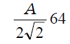
60 (negative frequency)

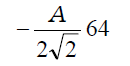
As in the previous example, substituting N = 64 and k = 4 into Equation (12) and performing the FFT yields the calculation results shown in Table 2. From these results, the amplitude is A using Equation (7), and the phase is −π/4 (= −45°) using Equation (8).

The signal component strength is displayed as an amplitude value (peak amplitude) or an RMS value, depending on the FFT analyzer settings. Since the phase also depends on data acquisition (the time window), sampling is generally synchronized to a specific timing point (using a trigger).

Next time, I’ll talk about power spectra.

[Keyword]

["Spectral analysis, Fourier analysis, Fourier series, Fourier transform, discrete Fourier transform (DFT), Fourier spectrum, amplitude spectrum, phase spectrum, complex Fourier coefficients, FFT, trigger"]

Reference Material

1. "Spectral Analysis" by Mikio Hino, Asakura Shoten (1977)

2. "Digital Fourier Analysis (I) - Basic Edition -" by Kenichi Kido, Corona Publishing (2007)

[Excerpt from the email newsletter issued on September 20, 2013]