Frequency Analysis from Basics (13) - 'Power Spectrum (Part 2)'

Signal Processing, FFT, and Frequency Analysis

Last time, I talked about the power spectrum (Part 1), which is the most basic and important function of the FFT analyzer as an electrical measuring instrument. This time, I will continue with the power spectrum (Part 2).

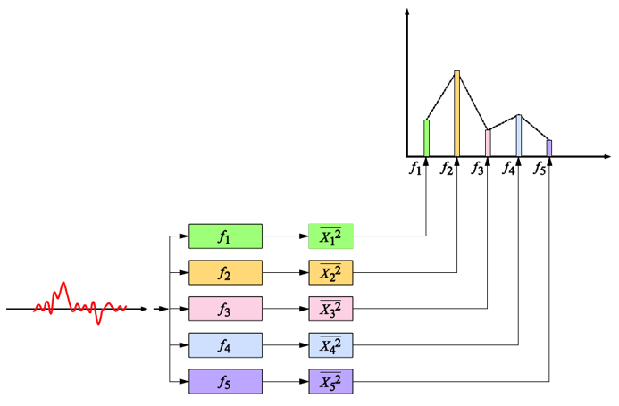
前回の繰り返しになりますが、パワースペクトルは、周波数の関数であり、元の時間信号に含まれる周波数毎のパワー(単位時間当たりのエネルギー)を表します。FFT アナライザでパワースペクトルを求める概念的な図を図 1 に示します。この図にあるようにフィルタを使って説明すると、FFT アナライザでパワースペクトルを求めることは、バンド幅が Δfの非常に急峻な L 個のフィルタ群(L は前回明した周波数軸上の分析ライン数で、例えば L= 800)に時間信号 x(t)を同時に通してその 2 乗平均値(パワー)を求めることと等価です。

(Note: This is not actual signal processing being performed by a real FFT analyzer.)

power spectrum

power

Frequency f

Band-pass filter
(bandwidth Δ f)

Root-mean-square circuit

Time-domain signal x(t)

図1 FFT アナライザでパワースペクトルを求める概念的な説明図

The issue here is the bandwidth Δf of the band-pass filter, which affects the power value. As explained in “Frequency Analysis from the Basics (8): The Discrete Fourier Transform (DFT),” periodic time signals have a discrete frequency distribution (line spectrum). Therefore, the power spectrum values of a periodic time signal are hardly affected (see Figure 2).

power

Frequency f

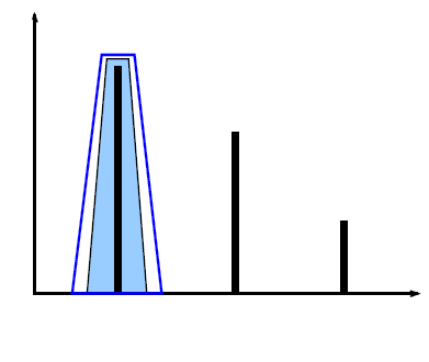
図2 バンド幅 Δf の違いに影響を受けないラインスペクトルのパワー値

それに対して、周期性のないランダム信号(不規則信号)のスペクトルは、連続スペクトルとなるので、分析するバンド幅 Δf によりそのパワー値は大きく変化します(図 3 のイメージ図参照)。例えば、バンド幅が 10 Hz の場合と 5 Hz の場合を比較すると、そのスペクトルの形状にもよりますが、10 Hz の方が 2 倍ほど大きくなります。この影響を最小化するために、通常は単位周波数(1 Hz 幅)当たりでパワー値を規格化します。この単位周波数(1 Hz 幅)で規格化されたスペクトル関数を、パワースペクトル密度関数(Power Spectral DensityFunction、以下 PSD)と呼びます。具体的には、前回のパワースペクトル(その 1)で説明したパワースペクトル P(k)の周波数分解能を Δf とすると、PSD G(k)は;

is required as.

power

Frequency f

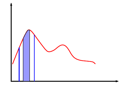
図3 連続スペクトルの分析バンド幅によるパワーの違い

The definition of PSD using the Fourier spectrum X(k) is as follows:

Therefore. For simplicity, the limits are omitted in the explanation below. As explained previously, X(k) is T times the complex Fourier coefficient c _k;

As shown in equation (4), the frequency resolution Δf is the inverse of the time window length T of the FFT.

We can see that Equation (3) is equal to Equation (1).

Just like the power spectrum P(k), the relationship between the mean square value (total power) of the time signal x(t) and the PSD G(k) is;

Therefore, by integrating the PSD, the mean square value of the time signal x(t) can be obtained.

PSD is used for evaluating an amplifier’s self-noise and for spectral profiles in random vibration testing. Its physical units are V ² /Hz, or, if an arbitrary physical quantity is denoted by EU, EU ² /Hz. In particular, when the physical quantity is vibration acceleration, it may also be called Acceleration Spectral Density (ASD). If acceleration is measured in m/s ², the unit of ASD is m ² /s ³.

In summary, the power spectral density function (PSD) represents the power (energy per unit time) per unit frequency (1 Hz width) contained in the original time signal as a function of frequency.

Next, we consider the case where the time signal x(t) is a finite time waveform, similar to an impulse waveform, rather than an infinite waveform.

As explained in “Frequency Analysis from the Basics (6) — Fourier Transform and Convolution,” |x(k)| ² in Equation (2) is the energy spectrum, while PSD represents the energy (power) per unit time. Therefore, it is divided by the FFT time-window length T. As a result, when calculating the PSD of an impulse waveform such as the one in Figure 4, the power values differ depending on the time-window lengths T ₁ and T ₂, for example. Thus, the calculated PSD is further multiplied by the time-window length T.

このように求められた周波数関数を、エネルギースペクトル密度関数(Energy SpectralDensity Function、以下 ESD)と呼びます。ESD を E(k)とすると;

ESD is used to determine the energy distribution of transient signals such as shock waveforms. Also, as with PSD, integrating ESD over the entire frequency band yields the total energy of the original time signal (the mean square value multiplied by T). Its physical units are V ² s/Hz, or EU ² s/Hz, where EU denotes any physical quantity.

As shown in Table 1 below, FFT analyzers utilize three types of spectra: power spectrum, PSD, and ESD, each within a given bandwidth.

Table 1 Comparison of Three Types of Spectra

types of spectra	physical meaning	the target signal	physical unit
power spectrum	Power distribution by frequency bandwidth.	periodic signal	EU²
PSD	Power distribution per unit frequency	continuous random signal	EU²/ Hz
ESD	Energy distribution per unit frequency	transitional signal	EU²s Hz

[Keyword]

Power spectrum, power, line spectrum, random signal, continuous spectrum, power spectral density function, PSD, acceleration spectral density, ASD, energy spectrum, energy spectral density function, ESD

Reference Material

"Spectral Analysis" by Mikio Hino, Asakura Publishing (1977 year)
"Digital Fourier Analysis (I)-Fundamentals-" by Kenichi Kido, Corona Publishing (2007 year)
"How to Use the Gentle FFT Analyzer" Edited by Yamaguchi and Ono, Ohmsha (1994 Year)

(Excerpt from the published email magazine dated January 23, 2014)

summary

Using an FFT analyzer to obtain the power spectrum is equivalent to simultaneously passing the time signal x(t) through a very steep filter group with an analysis bandwidth of Δf to calculate its 2 nd moment (power).
The spectrum of a periodic signal becomes a line spectrum, and its power value is not significantly affected by the analysis bandwidth, so a normal power spectrum can be applied.
The spectrum of a temporally continuous random signal becomes a continuous spectrum, and since the power values in the normal power spectrum depend on its analysis bandwidth, the power spectral density function (PSD) is applied.
Transient signals such as shock pulses are finite and their power values depend on the length of the analysis time window, so the energy density function (ESD) is applied.