

So far, we have discussed the fundamentals of vibration measurement over three installments. In this fourth installment, we will talk about the damping ratio.
The damping ratio ζ plays an important role in vibration behavior. In free vibration (Part 1), it affects whether vibration occurs and, if it does, how quickly it dies out. In forced vibration (Part 2), it affects the peak amplitude at the resonance frequency. In vibration transmissibility (Part 3), it affects both the peak amplitude at the resonance frequency and the transmissibility in frequency ranges above resonance.
In this installment (Part 4), we explain how to measure vibration using an FFT analyzer and determine the damping ratio ζ from the results.
There are various parameters used to express damping, depending on the field of application. First, we will introduce a method for calculating it from the logarithmic decrement.
The logarithmic decrement δ is defined as the natural logarithm of the ratio between adjacent amplitudes in the damped waveform of free vibration.
Why the natural logarithm? Of course, as shown in Figure 1, the amplitude of free vibration decays exponentially.
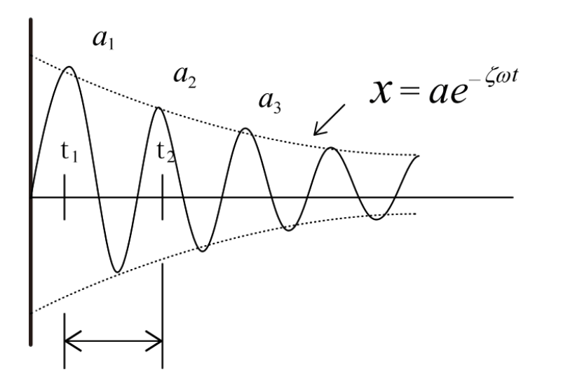
Figure 1: Damped Free Oscillation Waveform
The damped free-vibration waveform x(t) in Figure 1 is,
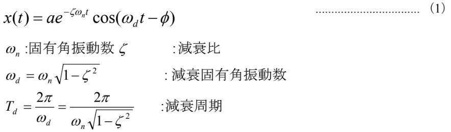
It becomes.
In Figure 1, the logarithmic decrement δ is
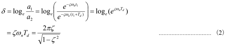
Here, if ζ ≪ 1

Next, to determine the logarithmic decrement δ, first use the Hilbert transform to obtain the envelope of the damped waveform, then plot time on the horizontal axis and the logarithm of the amplitude on the vertical axis (Figure 2).
-

Figure 2: Graph showing the envelope of the damped waveform with the vertical axis displayed in dB.
Since the logarithmic decrement δ is the slope with respect to the damped period T d, note that the dB scale uses the common logarithm; therefore, from the slope of the straight line in Figure 2,

Here, therefore

Using the Delta Search function of the FFT analyzer (DS-3000 Series), calculate the logarithmic decrement δ from equation (5).
Furthermore, from equation (3)

From the measured data and equation (5), the logarithmic decay rate δ can be calculated, and from equation (6), the damping ratio ζ can be determined.
Figure 3 shows an example where the damping time waveform of free vibration is measured by hammering, and then the logarithmic decay rate is calculated, followed by the determination of the damping ratio. Note that this figure utilizes the band-limiting function of the Hilbert transform to create a decay waveform for a single resonant frequency.
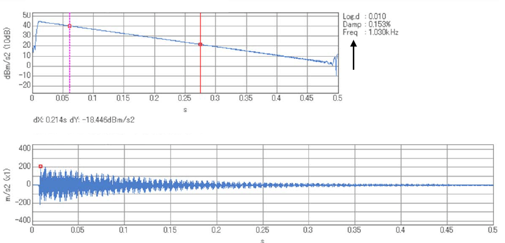
Figure 3: An example of calculating logarithmic decay rates and damping ratios from time waveform and envelope data.
Next, we will determine the damping ratio from the resonance peak of the frequency response function using the half-value width method.
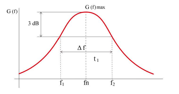
Figure 4: A diagram explaining the half-width method.
Let G(f) denote the frequency response function (compliance) of a single-degree-of-freedom system.

Here, f n: natural frequency ζ : damping ratio
In Figure 4, the points f1 and f2 are those where the resonant frequency fn is -3 dB (1/2 power and 1/√2 amplitude) from G(f)max, and Δf = f2-f1.
Since f1 and f2 can be expressed in modern terms as fn ± ∆f/2, the ratio with fn is

If you substitute this value into equation (7) and take the reciprocal,

Also, the maximum value is modernly than the style
 Because it becomes (9), when substituted into the equation.

Transform the equation

Because it uses the bandwidth at 1/2 power, the method for determining the damping ratio using equation (11) above is called the half-power bandwidth method.
In addition to the half-power bandwidth method, the mdB method can also be considered. In this case,

Here,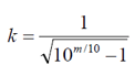
By the way, when it is 1 dB, k = 1.97; when it is 2 dB, k = 1.31.
The loss factor, used as an evaluation parameter for vibration damping materials, can also be determined using the full width at half maximum (FWHM) method. In damped vibrations with hysteretic damping, a complex modulus K' that generates a restoring force proportional to the vibration displacement is defined, with the real part as K1 and the imaginary part as K2.

Here,

This is the result. (Figure 5) This η is called the loss factor. The complex modulus K’ includes both the spring constant k and the viscous damping coefficient c in a single-degree-of-freedom system model. As shown in Figure 5, the loss factor is also called tan delta (tan δ).
-

Figure 5 Complex Elastic Modulus and Loss Factor
From the half-width method, the loss coefficient η can be calculated using the following formula.

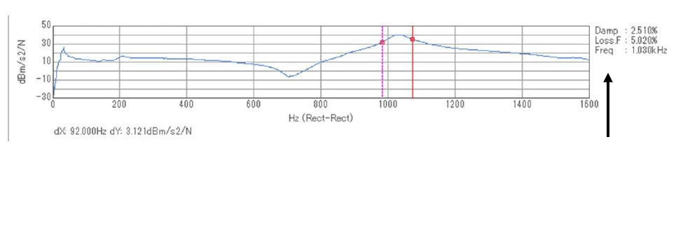
Figure 6 Empirical examples of damping ratios and loss coefficients measured by the half-width method.
Figure 6 shows an example of determining the damping ratio and loss coefficient from the FRF (Frequency Response Function) measured using the hammering method with an FFT analyzer, using the half-width method.
As a summary of various parameters, Table 1 below shows a list of the relationships between the various parameters that represent damping characteristics.
Table 1: Interrelationships Among Various Parameters
| Damping ratio ζ |
Logarithmic decrement δ |
Q value Q |
Loss factor η |
|
| z | — | 2πζ | 1 / 2ζ | 2ζ |
| δ | δ / 2π | — | π / δ | δ / π |
| Q | 1 / 2Q | π / Q | — | 1 / Q |
| η | η / 2 | πη | 1 / η | — |
Note 1: This table applies when ζ ≪ 1 can be assumed.
Note 2: The Q value is a measure of the sharpness of resonance when an oscillating system resonates, and is the reciprocal of the loss factor.
[Keyword]
damping ratio, free vibration, forced vibration, resonance frequency, vibration transmission rate, logarithmic decrement, natural angular frequency, damped natural angular frequency, damping period, Hilbert transform, envelope, delta search function, half-width method, half-power band width method, loss factor, complex modulus of elasticity, spring constant, viscous damping coefficient, tan delta, tandelta, hammering method, Q value
Reference
“Introduction to Modal Analysis,” by Akio Nagamatsu, Corona Publishing Co., Ltd. (1994)
Ono Sokki Technical Report, “Coefficients Representing Damping Characteristics”
(Excerpt from the newsletter published on January 21, 2016)


