

Last time, I talked about the power spectrum (Part 1), which is the most basic and important function of the FFT analyzer as an electrical measuring instrument. This time, I will continue with the power spectrum (Part 2).
To reiterate, the power spectrum is a function of frequency and represents the power (energy per unit time) at each frequency contained in the original time signal. Figure 1 shows a conceptual diagram of how to obtain a power spectrum using an FFT analyzer. As shown, explaining this using filters, obtaining a power spectrum with an FFT analyzer is equivalent to simultaneously passing the time signal x(t) through a bank of L very steep filters with a bandwidth of Δf (L is the number of analysis lines on the frequency axis explained previously, for example, L = 800) and calculating their mean-square values (power).
(Note: This is not actual signal processing being performed by a real FFT analyzer.)
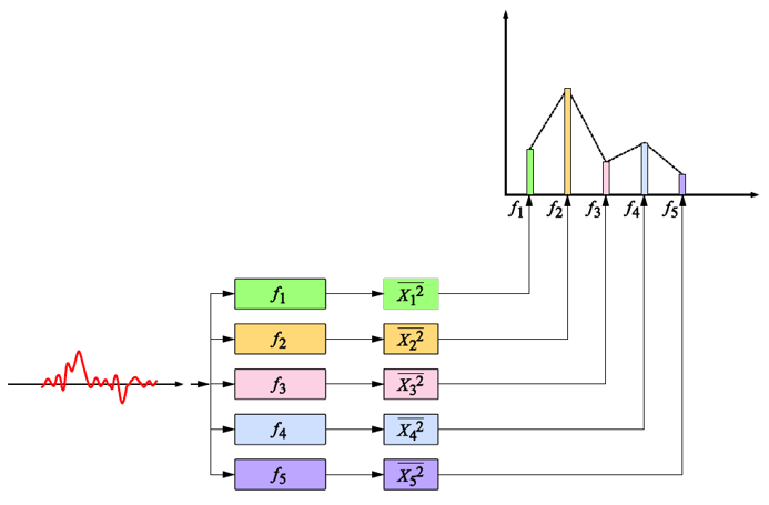
(bandwidth Δ f)
[{"source":"Figure 1: Conceptual diagram illustrating how to obtain a power spectrum using an FFT analyzer"}]
The issue here is the bandwidth Δf of the band-pass filter, which affects the power value. As explained in “Frequency Analysis from the Basics (8) — The Discrete Fourier Transform (DFT),” periodic time signals have a discrete frequency distribution (line spectrum). Therefore, the power spectral values of a periodic time signal are hardly affected (see Figure 2).
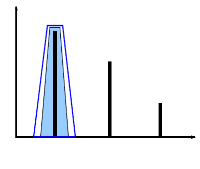
Figure 2. Power values of line spectra unaffected by differences in bandwidth Δf
In contrast, the spectrum of a random signal with no periodicity (an irregular signal) is continuous, so its power value varies considerably depending on the analysis bandwidth Δf (see the conceptual diagram in Figure 3). For example, comparing bandwidths of 10 Hz and 5 Hz, the value for 10 Hz will be about twice as large, depending on the shape of the spectrum. To minimize this effect, power values are usually normalized per unit frequency (1 Hz bandwidth). A spectral function normalized to this unit frequency (1 Hz bandwidth) is called the Power Spectral Density Function (hereafter PSD). Specifically, if the frequency resolution of the power spectrum P(k), described in the previous article, “Power Spectrum (Part 1),” is Δf, then the PSD G(k) is:

is required as.
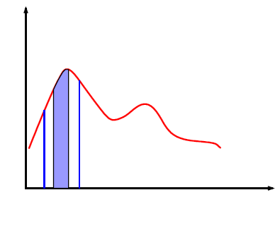
Figure 3. Power differences due to the analysis bandwidth of the continuous spectrum
The definition of PSD using the Fourier spectrum X(k) is as follows:

Therefore. For simplicity, the limits are omitted in the explanation below. As explained previously, X(k) is T times the complex Fourier coefficient c k;

As shown in equation (4), the frequency resolution Δf is the inverse of the time window length T of the FFT.

We can see that Equation (3) is equal to Equation (1).
Just like the power spectrum P(k), the relationship between the mean square value (total power) of the time signal x(t) and the PSD G(k) is;

Therefore, by integrating the PSD, the mean square value of the time signal x(t) can be obtained.
PSD is used for evaluating an amplifier’s self-noise and for spectral profiles in random vibration testing. Its physical units are V 2 /Hz, or, if an arbitrary physical quantity is denoted by EU, EU 2 /Hz. In particular, when the physical quantity is vibration acceleration, it may also be called Acceleration Spectral Density (ASD). If acceleration is measured in m/s 2, the unit of ASD is m 2 /s 3.
In summary, the power spectral density function (PSD) represents the power (energy per unit time) per unit frequency (1 Hz width) contained in the original time signal as a function of frequency.
Next, we consider the case where the time signal x(t) is a finite time waveform, similar to an impulse waveform, rather than an infinite waveform.
-

Figure 4. Finite shock waveform and the time-window length used to analyze it
As explained in “Frequency Analysis from the Basics (6) — Fourier Transform and Convolution,” |X(k)| 2 in Equation (2) is the energy spectrum, while PSD represents the energy (power) per unit time. Therefore, it is divided by the FFT time window length T. Consequently, when calculating the PSD of an impulse waveform such as the one in Figure 4, the power value differs depending on the time window, for example, T 1 and T 2. The calculated PSD is therefore multiplied by the time window length T.
The frequency function obtained in this way is called the Energy Spectral Density Function (hereafter ESD). If ESD is denoted by E(k);

ESD is used to determine the energy distribution of transient signals such as shock waveforms. Also, as with PSD, integrating ESD over the entire frequency band yields the total energy of the original time signal (the mean square value multiplied by T). Its physical units are V 2 s/Hz, or EU 2 s/Hz, where EU denotes any physical quantity.
As shown in Table 1 below, FFT analyzers utilize three types of spectra: power spectrum, PSD, and ESD, each within a given bandwidth.
Table 1 Comparison of Three Types of Spectra
|
types of spectra |
physical meaning |
the target signal |
physical unit |
|
power spectrum |
Power distribution by frequency bandwidth. |
periodic signal |
EU |
|
PSD |
Power distribution per unit frequency |
continuous random signal |
EU |
|
ESD |
Energy distribution per unit frequency |
transitional signal |
EU |
[Keyword]
Power spectrum, power, line spectrum, random signal, continuous spectrum, power spectral density function, PSD, acceleration spectral density, ASD, energy spectrum, energy spectral density function, ESD
Reference Material
- "Spectral Analysis" by Mikio Hino, Asakura Publishing (1977 year)
- "Digital Fourier Analysis (I)-Fundamentals-" by Kenichi Kido, Corona Publishing (2007 year)
- "How to Use the Gentle FFT Analyzer" Edited by Yamaguchi and Ono, Ohmsha (1994 Year)
(Excerpt from the published email magazine dated January 23, 2014)


